Chapter 1: Introduction

Welcome to the User Manual for Replay Test Engine, your regression and verification testing tool designed to enhance the quality and reliability of developments and configuration changes within the SAP software ecosystem. This manual is intended for SAP developers, Functional Consultants, QA testers, and Key Users involved in testing SAP program modifications or verifying the impact of configuration adjustments.

The dynamic nature of SAP systems, with frequent enhancements, bug fixes, customizations, and configuration updates, carries an inherent risk: changes intended to improve one area can inadvertently impact other, seemingly unrelated functionalities. Ensuring that modifications deliver their desired benefits without introducing new errors or regressing existing features is paramount for maintaining system stability, user trust, and business continuity. RTE directly addresses this critical challenge by providing a structured, efficient, and powerful framework for conducting comprehensive regression testing of your SAP programs and verification of configuration outcomes.

1.1 Purpose of RTE

The primary purpose of RTE is to empower all teams to verify that modifications made to SAP programs, or changes to system configuration, have not negatively impacted their output for specific, well-defined scenarios. It achieves this by allowing you to:

• Capture a Baseline: Precisely record the state of key program variables before any code or configuration changes are applied. This "reference run" acts as your trusted baseline, representing the correct and expected behaviour.
• Execute and Compare: After program modifications or configuration updates, re-execute the program and use RTE's robust comparison engine to automatically identify any deviations from the established reference.
• Analyse and Adapt: Investigate identified differences with detailed insights and, when necessary, utilize advanced data mapping capabilities to handle intentional structural changes or compare against different programs.

By systematically comparing "before" and "after" states, RTE helps you catch regressions early in the cycle, reducing the cost and effort associated with fixing issues later.

1.2 The RTE Workflow

At its heart, RTE operates on the principle of structured comparison, integrated directly into your development, configuration, and testing lifecycle. The typical workflow involves several key stages:

1. Instrumentation: Identify the critical internal variables within your SAP program (custom or standard) whose state you need to monitor. This is achieved with minimal code intrusion, typically by adding a single line of ABAP code using static methods from the ZCL_RTE class (ZCL_RTE=>EXPORT_DATA). This can often be done via a simple enhancement, requiring only very basic ABAP knowledge. You can also optionally use methods like ZCL_RTE=>IN_RTE() for test-specific logic or ZCL_RTE=>COMBINE_DATA() to enrich data before export.
2. Creating Reference Runs: Access the central RTE transaction (ZRTE_START) and use the "Run program" function. Execute your instrumented program before applying any changes (or with a known 'good' configuration), using specific program variants to ensure consistent results. Mark these initial executions as "reference runs". These runs encapsulate the expected, correct output for those scenarios.
3. Implementing Program or Configuration Changes: Proceed with your development activities or configuration adjustments.
4. Performing Comparisons: Return to ZRTE_START and use the "Compare runs" function. RTE offers several modes:
   • Re-run the modified program for a specific variant and compare it against its reference.
   • Re-run for all reference variants and compare each against its baseline.
   • Compare any two arbitrary historical runs.
5. Analysing Results: RTE will highlight any discrepancies in output (raw data differences, structural changes, or detailed content variations if using iData comparison). If intentional structural changes were made to your data, or if you're performing a cross-check against a different program, RTE's advanced "iData parameters" allow for sophisticated data mapping (renaming fields, changing types, filtering rows, etc.) to enable meaningful comparison.
6. Managing and Approving Runs: Use "Manage runs" to view or delete old test data. Crucially, after verifying that the output of a modified program or new configuration is correct, you can "Approve" the new runs within the comparison tool, promoting them to become the new reference baseline for future tests.

1.3 About This Manual

This manual guides you through all features of RTE. It assumes basic SAP navigation skills. While Chapter 2 discusses code, instrumenting standard programs for configuration checks is designed to be accessible even with minimal ABAP exposure. Key Users can often leverage RTE for programs already instrumented by developers or consultants.

Chapter 2: Defining Test Data

To enable RTE to perform comparisons, you first need to instruct it which data within an SAP program (custom or standard) should be captured during a test run. This is achieved by adding a small amount of code directly into the program you intend to test. The integration is designed to be straightforward, primarily using static methods from the global class ZCL_RTE, which means you can call them easily without needing to declare helper variables.

2.1 Exporting Data for Comparison

The core mechanism for identifying test data is the EXPORT_DATA method. By calling this method, you specify an internal variable (like an internal table or a structure) whose content RTE should save when the program is executed via the RTE tool.

The simplest way to use this is with a single line of code:

ZCL_RTE=>EXPORT_DATA( iv_var_name = 'LT_OUTPUT_TAB' i_data = <lt_tab> ).

Let's break down the parameters:

• IV_VAR_NAME : (Input, Type CHAR30) This is the logical name you assign to the data being exported. This name will be displayed within the RTE tool during comparison setup and results viewing. Important: This name does not have to match the actual ABAP variable name in your program. Choose a descriptive name that makes sense in the context of your test (e.g., 'FINAL_OUTPUT_TABLE', 'HEADER_DATA').
  • Important: The logical name provided in the IV_VAR_NAME parameter must adhere to standard ABAP variable naming rules. It should primarily consist of letters and numbers. The following special characters are also permitted: underscore (_), exclamation mark (!), percentage sign (%), dollar sign ($), ampersand (&), and asterisk (*). Avoid other special characters or spaces.
  • Warning: When multiple EXPORT_DATA calls are made within a single program execution (one test run), ensure that the IV_VAR_NAME used for each distinct data element is unique. If you assign the same logical name (IV_VAR_NAME) to two or more different actual variables (I_DATA) within the same run, RTE will not raise an explicit error. However, the data associated with that name within the run record will likely be overwritten or combined unpredictably, leading to corrupted or meaningless results during comparison. If exporting the same variable multiple times (e.g., in a loop to see its state at different points), RTE uses the ZRTE_UNIQN field (see section 2.3) to differentiate these snapshots.
• I_DATA : (Input, Type ANY) This is the actual data object (internal table, structure, elementary variable) from your program that you want RTE to capture and save for comparison. Pass the variable itself here.
  • Warning: The ZCL_RTE=>EXPORT_DATA method is designed to capture standard data types. It fully supports elementary variables, flat structures and internal tables. Complex objects (instances of classes), data references, or nested internal tables (tables containing other tables directly as line items) are not supported for export via I_DATA.
• IV_CPROG : (Optional Input, Type SYST-CPROG, Default SY-CPROG) This parameter allows you to explicitly specify the program name under which the data should be stored in RTE. This is typically only necessary in specific scenarios, such as when testing a program that is submitted via SUBMIT REPORT by another wrapper program. In most cases, you can omit this parameter, and RTE will automatically determine the correct program name.

Example Placement:

You should place the EXPORT_DATA call at a point in your program's logic where the variable you want to test contains the final data relevant for your comparison. Often, this is near the end of the program or subroutine, after all processing and data preparation for that variable is complete.

Consider this typical example where data is exported just after being displayed using ALV:

  " ... preceding program logic ...
  lo_alv_table->display( ).

  ZCL_RTE=>EXPORT_DATA( iv_var_name = 'FINAL_ALV_DATA' i_data = gt_data ).
ENDFORM.

2.1.1 Instrumenting Standard SAP Programs

RTE can also be used to verify the impact of configuration changes. You can instrument standard SAP programs by adding an EXPORT_DATA call using SAP's Enhancement Framework. This is often a very simple process requiring minimal ABAP knowledge, making it accessible to Functional Consultants.

• How it Works:
  1. Identify a standard SAP program or function module whose output is affected by the configuration you are changing.
  2. Find a suitable enhancement point/spot (often at the end of a subroutine or function module, after the relevant data has been processed).
  3. Create a simple source code enhancement implementation.
  4. Add a single ZCL_RTE=>EXPORT_DATA(...) line to export the key internal table or structure that reflects the configuration's outcome.
• Benefit: This allows you to capture the "before" state of a standard process, make your configuration changes, then capture the "after" state and use RTE to precisely identify what changed, ensuring the configuration works as intended and hasn't had unforeseen side effects.

2.2 Manipulating Data for Testing

Sometimes, the raw data in your program variables might not be in the ideal format for comparison, or you might want to include additional context only during test runs. RTE provides helper methods to handle these situations without affecting the standard execution flow of your program.

2.2.1 Conditional Logic

To execute specific data preparation steps only when the program is being run as part of an RTE test, you can use the IN_RTE method.

• Method: ZCL_RTE=>IN_RTE( )
• Parameters: None
• Returns: abap_bool (abap_true if running within RTE, abap_false otherwise).

You can wrap your test-specific data manipulation logic within an IF ZCL_RTE=>IN_RTE( ) EQ abap_true...ENDIF. block. This ensures that this code is completely bypassed during normal program operation.

2.2.2 Merging Data

A common requirement is to combine data from different sources before exporting it for comparison. For instance, you might want to add a specific field as an extra column to every row of an internal table being tested. The COMBINE_DATA method facilitates this. Note: This method supports adding fields from a structure or elementary variable to a base table or structure; combining two tables is not supported.

• Method: ZCL_RTE=>COMBINE_DATA( ... )
• Parameters:
  • I_A_TAB_OR_STR : (Input, Type ANY) The base internal table or structure to which you want to add data.
  • IT_A_FIELDS : (Optional Input, Type Range Table for Field Names) A range table specifying which fields from "I_A_TAB_OR_STR" should be included in the output. If omitted, all fields are used.
  • I_B_STR_OR_ELEM : (Input, Type ANY) The structure or elementary variable containing the data you want to add.
  • IT_B_FIELDS : (Optional Input, Type Range Table for Field Names) A range table specifying which fields from "I_B_STR_OR_ELEM" should be added to the output. Use this to select specific fields if "I_B_STR_OR_ELEM" is a structure.
  • E_TAB : (Output, Type REF TO DATA) A data reference that will point to the newly created internal table containing the combined data.

Example: Combining a Table with a System Field for Testing

Let's look at how to use IN_RTE and COMBINE_DATA together. Imagine you want to test the contents of table gt_usr, but for testing purposes, you also want each row to include the System ID (sy-sysid).

  IF ZCL_RTE=>IN_RTE( ) EQ abap_true.

    ZCL_RTE=>COMBINE_DATA(
      EXPORTING
        i_a_tab_or_str  = gt_usr    " Base table or strucure
*       it_a_fields     =           " Fields to be used in output
        i_b_str_or_elem = sy        " Structure or elemtary var to be added
        " Fields to be used in output
        it_b_fields     =  VALUE #( (  sign = 'I' option = 'EQ' low = 'SYSID' ) )
      IMPORTING
        e_tab           =  DATA(go_ref) " Combined table
    ).

    FIELD-SYMBOLS: <gt_tab> TYPE ANY TABLE.
    ASSIGN go_ref->* TO <gt_tab>.

    ZCL_RTE=>EXPORT_DATA( iv_var_name = 'GT_TAB_WITH_SYSID' i_data = <gt_tab> ). " Ensure unique IV_VAR_NAME

  ENDIF.

Explanation of the Example:

1. Check Execution Mode: IF ZCL_RTE=>IN_RTE( ) EQ abap_true. ensures the combination logic runs only during RTE tests.
2. Combine Data: ZCL_RTE=>COMBINE_DATA is called:
   • gt_usr is the base table.
   • sy structure provides the additional data.
   • it_b_fields specifically selects only the SYSID field from the sy structure to be added.
   • The result (a new table combining gt_usr fields and sy-sysid) is created, and go_ref points to it.
3. Export: ZCL_RTE=>EXPORT_DATA is called using the field symbol. It exports the combined data during an RTE run under a distinct logical name.

By using these methods, you can precisely define and even adapt the data captured by RTE for effective regression testing, without impacting the program's behaviour for end-users.

2.2.3 Real-World Example

While the COMBINE_DATA method can be used for various data manipulations, a common and powerful use case is adding contextual information to a primary data table before exporting it for testing. This makes test results much easier to analyze, especially when dealing with data processed in loops or across different entities (like employees, materials, documents, etc.). This technique is also valuable for configuration verification, for instance, to check payroll results before and after a configuration change with an effective date.

Let's consider a scenario from SAP Payroll. Within the standard payroll driver, the EXPRT function processes the Results Table (RT) for each employee (PERNR) and payroll period (APER). For regression testing or configuration verification, simply exporting the RT table might not be sufficient, as you wouldn't immediately know which employee or period a specific RT entry belongs to when looking at the combined test results later.

The following code snippet, intended to be placed within the relevant part of the payroll logic (like function EXPRT, potentially via an enhancement for standard code), demonstrates how to use ZCL_RTE=>COMBINE_DATA twice to add both the employee number and the payroll period information as columns to the RT table, specifically for RTE test runs:

FIELD-SYMBOLS: <lt_tab>  TYPE ANY TABLE,
               <lt_tab2> TYPE ANY TABLE.


IF ZCL_RTE=>IN_RTE( ) EQ abap_true.

  " Step 1: Combine RT table with the Personnel Number (PERNR)
  ZCL_RTE=>COMBINE_DATA(
    EXPORTING
      i_a_tab_or_str  = rt[]      " Base table is RT
      i_b_str_or_elem = pernr     " Add data from PERNR structure
      " Select only the 'PERNR' field from the PERNR structure
      it_b_fields     = VALUE #( ( low = 'PERNR' sign = 'I' option = 'EQ' ) )
    IMPORTING
      e_tab           = DATA(l_out_data) " Output: RT fields + PERNR field
  ).

  ASSIGN l_out_data->* TO <lt_tab>. " Assign intermediate result

  " Step 2: Combine the intermediate table with the Payroll Period (APER)
  ZCL_RTE=>COMBINE_DATA(
    EXPORTING
      i_a_tab_or_str  = <lt_tab>   " Base table is the result from Step 1
      i_b_str_or_elem = aper      " Add data from APER structure
      " IT_B_FIELDS is omitted, so add ALL fields from APER structure
    IMPORTING
      e_tab           = DATA(l_out_data2) " Output: RT fields + PERNR field + APER fields
  ).

  ASSIGN l_out_data2->* TO <lt_tab>. " Assign final result

  " Step 3: Export the final combined table
  ZCL_RTE=>EXPORT_DATA(
    EXPORTING
      iv_var_name = 'RT_DATA'       " Logical name for the exported data
      i_data      = <lt_tab2>       " The table containing RT + PERNR + APER
  ).
ENDIF.

Explanation:

1. IF ZCL_RTE=>IN_RTE( )...ENDIF. : This ensures the entire data combination logic executes only when the program is run via RTE, having no impact on regular payroll runs.
2. First COMBINE_DATA Call :
   • Takes the current RT internal table (i_a_tab_or_str = rt[]).
   • Adds data from the PERNR structure (i_b_str_or_elem = pernr).
   • Crucially, it_b_fields specifies that only the field named 'PERNR' from the pernr structure should be added as a new column to each row of the RT table.
   • The result is a new table (referenced by l_out_data, assigned to <lt_tab>) containing all original RT fields plus a PERNR field.
3. Second COMBINE_DATA Call :
   • Takes the intermediate table <lt_tab> (which already contains RT + PERNR) as the base (i_a_tab_or_str = <lt_tab>).
   • Adds data from the APER structure (i_b_str_or_elem = aper).
   • Since it_b_fields is not provided this time, all fields from the aper structure are added as new columns to the table.
   • The result is the final table (referenced by l_out_data2, assigned to <lt_tab2>) containing original RT fields, the PERNR field, and all fields from the APER structure.
4. EXPORT_DATA Call : The final, enriched table <lt_tab2> is exported under the logical name 'RT_DATA'.

Outcome and Applicability:

By performing these combinations before the export, the 'RT_DATA' variable captured by RTE will contain not just the payroll results but also the associated employee number and period details directly within each row. This makes analyzing differences during comparison significantly easier, as the context is immediately apparent.

Universal Technique: While this specific example uses variables common in SAP Payroll (RT, PERNR, APER), the underlying technique is universally applicable. You can use ZCL_RTE=>IN_RTE and ZCL_RTE=>COMBINE_DATA in any SAP module to enrich your primary test data with relevant contextual information (like document numbers, material codes, company codes, dates, etc.) before exporting it with ZCL_RTE=>EXPORT_DATA, thereby enhancing the clarity and usefulness of your regression tests or configuration verifications.

2.3 Exporting Different Variable Types

Let's examine an example demonstrating how to export variables of different types (elementary variable, structure, and internal table) using ZCL_RTE=>EXPORT_DATA. This example also illustrates how RTE handles situations where the same logical variable name (IV_VAR_NAME) is exported multiple times within a single program execution, such as within a loop.

Consider the following ABAP code snippet:

DATA: lv_var TYPE string,
      ls_str TYPE t000,
      lt_tab TYPE TABLE OF usr02.

lv_var = 'Single variable'.
SELECT SINGLE * FROM t000 INTO @ls_str WHERE mandt = '000'.
SELECT * FROM usr02 INTO TABLE @lt_tab.

DO 3 TIMES.
  " Modify variables slightly in each loop iteration
  lv_var = lv_var && '__' && sy-index.
  ls_str-mtext = ls_str-mtext && '__' && sy-index.
  READ TABLE lt_tab ASSIGNING FIELD-SYMBOL(<ls_tab>) INDEX 1.
  IF sy-subrc EQ 0.
    <ls_tab>-accnt = sy-index. " Change only one field in the first row of the table
  ENDIF.

  " Export all three variables in each iteration
  ZCL_RTE=>EXPORT_DATA( iv_var_name = 'LV_VAR' i_data = lv_var ).
  ZCL_RTE=>EXPORT_DATA( iv_var_name = 'LS_STR' i_data = ls_str ).
  ZCL_RTE=>EXPORT_DATA( iv_var_name = 'LT_TAB' i_data = lt_tab ).

ENDDO.

In this code:

• We declare a string (lv_var), a structure (ls_str based on T000), and an internal table (lt_tab based on USR02).
• We initialize these variables with some data.
• We loop three times (DO 3 TIMES.).
• Inside the loop, we slightly modify the content of each variable in each iteration.
• Crucially, within each loop iteration, we call ZCL_RTE=>EXPORT_DATA for all three variables, using the same IV_VAR_NAME ("LV_VAR", "LS_STR", "LT_TAB") respectively across iterations.

Viewing the Exported Data in RTE:

After executing this code via the "Run program" function in RTE, if you inspect the captured data for this run (as described in Chapter 4.4), you will observe the following:

1. Elementary Variable (LV_VAR):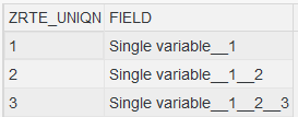
   • Since LV_VAR is an elementary variable (string), its value is displayed in a single column with the generic header FIELD.
   • Notice the ZRTE_UNIQN column. This field acts as a unique identifier for each distinct call to ZCL_RTE=>EXPORT_DATA within the run for the same IV_VAR_NAME. Because EXPORT_DATA for "LV_VAR" was called three times (once per loop iteration), you see three rows, each with a different ZRTE_UNIQN value (1, 2, 3), reflecting the state of lv_var at the moment of each export.
2. Structure (LS_STR):
   • For the structure LS_STR, RTE displays the data using column headers that directly correspond to the field names of the T000 structure (e.g., MANDT, MTEXT, ORT01, etc.).
   • Similar to the elementary variable, the ZRTE_UNIQN column appears, again having distinct values (1, 2, 3) for each of the three times EXPORT_DATA was called for 'LS_STR', showing the state of the structure in each loop pass.
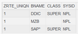
3. Internal Table (LT_TAB):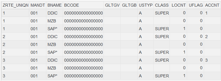
   • When viewing the internal table LT_TAB, the column headers correspond to the fields of the table's line type (USR02, e.g., MANDT, BNAME, ACCNT, etc.).
   • Here, the role of ZRTE_UNIQN becomes particularly clear. The internal table (lt_tab) contains multiple rows itself. RTE exports the entire table contents each time ZCL_RTE=>EXPORT_DATA is called for 'LT_TAB'.
   • Therefore, you will see multiple groups of rows in the display, each group corresponding to a single export call. The ZRTE_UNIQN value will be the same for all rows belonging to a single export call (one snapshot of the table), but it will differ between the export calls made in different loop iterations. In this example, all table rows exported during the first loop pass will have ZRTE_UNIQN = 1, all rows from the second pass will have ZRTE_UNIQN = 2, and all from the third pass will have ZRTE_UNIQN = 3. This allows you to distinguish the complete state of the table as it was captured at each specific export moment. You can also see the effect of the modification within the loop: the ACCNT field for the first user (DDIC in the screenshot) changes value (1, 2, 3) corresponding to the ZRTE_UNIQN identifier for that export set.

This example highlights how RTE handles different data types and preserves the state of variables even when exported multiple times under the same logical name within a single execution, using the ZRTE_UNIQN field to differentiate between these distinct export snapshots.

2.4 Data Storage

Internally, when ZCL_RTE=>EXPORT_DATA is called, the content of the provided variable (I_DATA) is serialized into a raw data format. This serialized representation is then saved persistently, within dedicated database tables managed by the RTE tool. For complex types like internal tables or structures, this process typically involves converting each row of the variable into its raw data equivalent, and this will result in each field or cell of the source variable being stored as a distinct record or part of a record in the RTE backend tables, along with metadata such as the run identifier, logical variable name, and export sequence (ZRTE_UNIQN).

Chapter 3: The Central RTE Transaction

Once you have instrumented your program(s) by adding the necessary ZCL_RTE=>EXPORT_DATA calls (as described in Chapter 2), the next step is to interact with the RTE tool itself to create runs and perform comparisons. The primary access point for all RTE functionalities is the central transaction ZRTE_START.

3.1 Accessing the RTE Main Screen

To begin using the RTE tool's interactive features, navigate to the SAP transaction ZRTE_START. You will be presented with the main screen, titled "RTE - Replay Test Engine", which serves as the central hub for managing your regression testing and configuration verification activities.

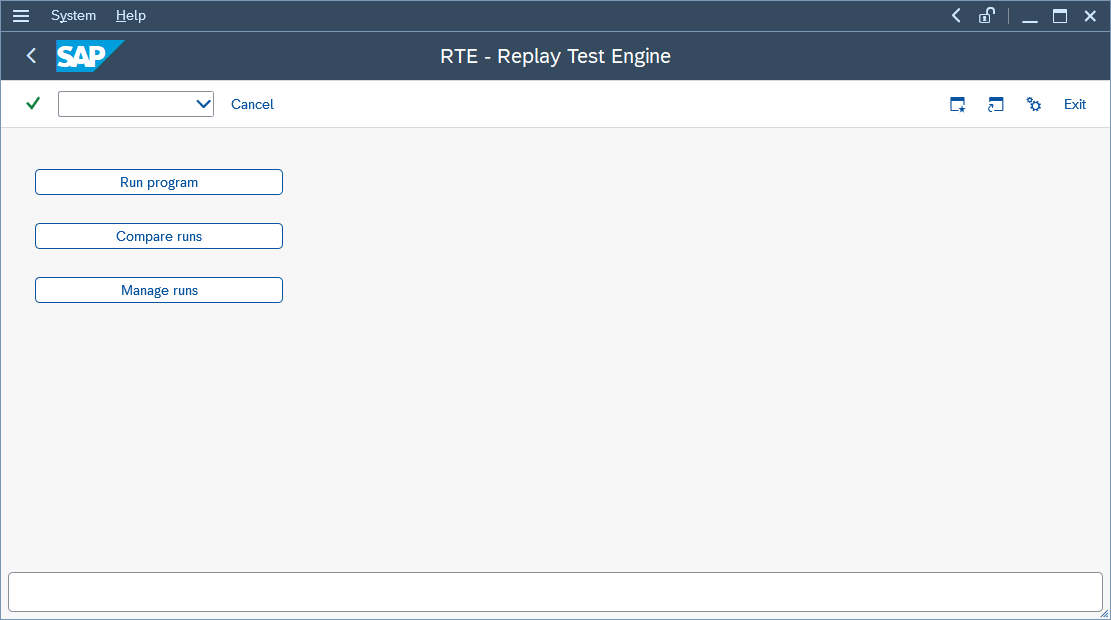
3.2 Overview of Main Functions

The ZRTE_START transaction provides direct access to the core components of the RTE solution through three main options:

1. Run program: This function is used to execute your instrumented SAP program (custom or standard) under specific conditions (usually with a predefined variant) and capture the data you marked for export using ZCL_RTE=>EXPORT_DATA. Each execution creates a "run" record within RTE, storing the captured data and associated context (like program name, variant, timestamp, user, and an optional description). These runs form the basis for later comparisons. You will typically use this to create your reference runs before making changes (code or configuration) and subsequent runs after making changes.
2. Compare runs: This is the heart of the RTE tool. This function provides a powerful interface for comparing the data captured in different runs. You can compare a recent run against a reference run of the same program, compare two arbitrary runs, or even compare a run against the output of a different program (cross-program testing). This section offers various comparison modes and advanced data mapping capabilities to pinpoint differences effectively.
3. Manage runs: This utility allows you to view, search for, and maintain the test runs that have been previously created. You can search for runs based on various criteria (like program name, variant, user, date, or description), preview the data captured within a specific run, and delete runs that are no longer needed.

3.3 Navigating This Manual

The subsequent chapters of this manual will delve into the detailed usage of each of these core functions ("Run program", "Compare runs", and "Manage runs"), explaining their features, options, and workflows step-by-step. You will typically start by creating runs using "Run program", and then analyze the results using "Compare runs".

Chapter 4: Creating Test Runs

The first step in the practical application of RTE is typically to create one or more "runs" of the program you intend to test. A run represents a single execution via RTE, during which the tool captures the data you designated using the ZCL_RTE=>EXPORT_DATA method. These saved runs are the essential building blocks for later comparisons.

To create a run, select the "Run program" option from the main ZRTE_START transaction screen (described in Chapter 3). This will navigate you to the "RTE: Run program" screen.

4.1 Specifying Run Parameters

On the "RTE: Run program" screen, you need to provide details about the execution you want to perform:

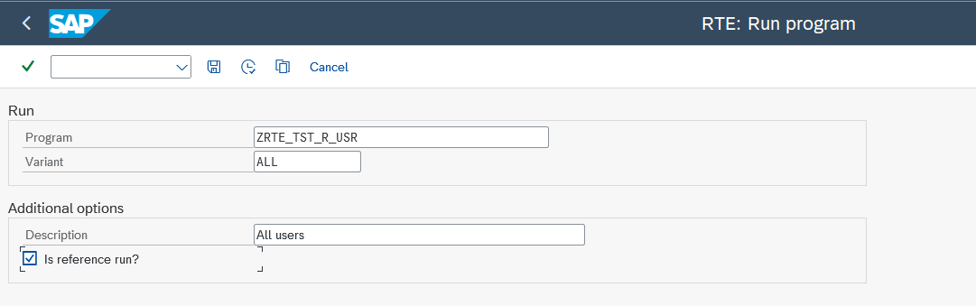
• Program: Enter the technical name of the SAP report (program) you wish to execute (e.g., ZRTE_TST_R_USR). Important: This should be the report name, not the transaction code that might normally be used to start it.
• Variant: Specify the execution variant you want to use for this run.
  • It is highly recommended to use a saved variant. Using variants ensures that the program runs with the exact same selection criteria and parameters each time, which is crucial for achieving repeatable and reliable test results for both code and configuration checks.
  • Real-World Scenarios & Coverage: Variants used for testing should reflect real-life scenarios as closely as possible, utilizing anonymized production data on development and quality systems if only possible. The more variants (and thus reference runs) created, the more comprehensive the code coverage. As you prepare more tests and variants, you increase the overall test coverage.
  • Skipping Variant: If you leave the "Variant" field blank, RTE will display the program's standard selection screen when you execute the run (if one exists). You can then enter parameters manually. However, this approach makes it harder to guarantee test repeatability, as manual input can vary between runs.
  • It's important to note that while using variants is highly recommended for programs with selection screens to ensure test repeatability, some SAP programs are designed without a selection screen altogether. For such programs, leaving the "Variant" field blank in the "RTE: Run program" screen is the correct and necessary procedure to execute them via RTE. In these cases, the tool will directly execute the program without attempting to display a selection screen.
• Description: (Optional) Provide a meaningful description for this run. This text will help you identify the run later when managing runs or setting up comparisons (e.g., "Baseline before performance tuning," "Run after defect fix #123," "Sales Pricing - Before ZNEW activation," "Payroll - Jan 2024 - Pre-config change").
• Is reference run?: (Checkbox) This is a critical option.
  • Check this box if this specific run represents the correct, expected output against which future runs (after code or configuration changes) should be compared. Typically, you create reference runs before making modifications.
  • Uniqueness Constraint: For any given combination of Program and Variant, only one run can be marked as the reference run at any time.

4.2 Handling Existing Reference Runs

Because only one reference run is allowed per program/variant pair, if you check the "Is reference run?" box and a reference run already exists for the specified Program and Variant, RTE will prompt you for confirmation:

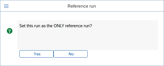
• Confirmation: The pop-up asks: "Set this run as the ONLY reference run?".
• If you choose "Yes", the current run you are creating will be marked as the new reference run, and the previously existing reference run for this program/variant combination will automatically have its reference flag removed.
• If you choose "No", the current run will still be created, but it will not be marked as a reference run, even though you initially checked the box on the selection screen. The existing reference run will remain unchanged.

4.3 Executing the Run

Once you have filled in the parameters, execute the run (by pressing F8 or clicking the Execute icon). RTE will launch the specified program with the selected variant (or display the selection screen if no variant was provided). The program will execute, and the ZCL_RTE=>EXPORT_DATA calls within its code (or enhancement) will trigger RTE to capture the specified variables.

After the program execution finishes, RTE will display a summary screen showing the variables that were successfully exported during this run:

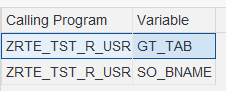
This list shows the logical variable names (Variable column) you defined using the IV_VAR_NAME parameter in your ZCL_RTE=>EXPORT_DATA calls, along with the program they originated from.

Disclaimer: Handling Runtime Errors (Short Dumps). Please be aware that RTE executes the target program as is. If the program encounters a runtime error (short dump) during its execution initiated by RTE, the execution will terminate, and the run will likely not be saved completely or correctly. RTE does not include mechanisms to catch or handle these short dumps. This applies even if the runtime error is potentially caused by incorrect usage of ZCL_RTE methods (e.g., passing incompatible data types to EXPORT_DATA or COMBINE_DATA). Ensuring the stability of the program under test, including the correct implementation of RTE method calls (whether in custom code or enhancements), remains the responsibility of the developer initiating the run. Check transaction ST22 for dump details if this occurs.

4.4 Inspecting Captured Data

You can immediately inspect the data captured for any variable listed. Simply double-click on the row corresponding to the variable you want to view. RTE will then display the content of that variable (in read-only mode) as it was saved during the run.

This allows for a quick verification that the expected data was captured correctly.

This run, along with the captured data, is now saved within the RTE system and can be used for comparisons (see Chapter 5) or managed via the "Manage runs" function (see Chapter 6).

Chapter 5: Comparing Test Runs

Having successfully instrumented your programs (Chapter 2) and captured baseline executions as runs (Chapter 4), we now arrive at the central purpose and most powerful aspect of the RTE tool: comparing these runs. This is where RTE truly shines, allowing you to analyze the effects of your code modifications or verify the outcomes of configuration changes, ensuring that enhancements deliver the intended value without introducing unintended side effects. This chapter will guide you through the different ways to initiate comparisons, the various types of analysis RTE can perform, and data mapping features that enable meaningful comparisons even when program structures evolve.

5.1 Understanding the Modes

We start the comparison on the "RTE: Compare runs" screen, where you must first decide how you want RTE to select the runs for comparison. RTE offers three distinct operational modes, each suited to different testing scenarios:

1. Reference program/variant:
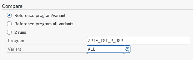
   • Core Idea: This mode focuses on validating a single, specific test scenario after code or configuration changes. You pinpoint the exact Program and Variant you are interested in testing.
   • How it Works: RTE locates the unique reference run previously saved for this specific program/variant combination. Then, crucially, it triggers a fresh execution of the current version of the specified program (with its current code and system configuration) using that same variant. Finally, it compares the data exported during this new execution against the data stored within the historical reference run.
   • Prerequisite: A reference run must already exist for the chosen program and variant. If not, RTE will issue a notification, and no comparison can proceed for that specific selection. Convenient search helps are available, first for selecting the Program, and then for listing only the valid Variants associated with that program.
2. Reference program all variants:
   • Core Idea: This mode offers a broader safety net, automatically testing all established reference scenarios for a given program in one go. You only need to specify the Program name.
   • How it Works: RTE scans its records to find every variant associated with the entered Program name for which a reference run has been previously created. For each of these identified variants, it performs the same process as the single variant mode: it re-executes the program with that variant and compares the new results against the corresponding reference run.
   • Typical Use Case: This is the ideal mode for comprehensive regression testing after program changes. It provides assurance that your modifications haven't broken functionality across any of the standard test scenarios you've established as references. It's thorough but may take longer if many reference variants exist.
3. 2 runs:
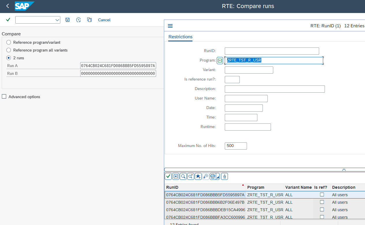
   • Core Idea: This mode grants complete manual control, allowing you to select any two previously completed runs from the RTE history for a direct comparison.
   • How it Works: You explicitly provide the unique technical identifiers (Run IDs) for the two runs you wish to compare, designated as "Run A" and "Run B". RTE then retrieves the data stored for these specific runs and performs the comparison.
   • Selecting Runs: The Run IDs themselves are long, system-generated strings and not easily remembered. Therefore, RTE provides search helps for both the "Run A" and "Run B" fields. These search helps allow you to locate the desired runs using familiar criteria such as the Program name, Variant used, the Description you provided during run creation, the User who created the run, or the Date/Time of execution.

5.2 Practical Scenarios Setup

To make the comparison features easy to follow, we'll use a concrete example throughout this chapter. We'll base our examples on the sample program ZRTE_TST_R_USR, which is provided as part of the RTE tool package (you are encouraged to copy this program into your own Z*-namespace program to experiment alongside this manual). This program's core function is to display user information from the standard SAP table USR02. While simple, it's perfectly sufficient to demonstrate RTE's comparison capabilities.

Initial Preparation Steps:

1. Variant Creation: Define and save three distinct variants for your ZRTE_TST_R_USR program:
   • ALL Selection Criteria: Leave all selection fields blank (this will select all users).
   • DS Selection Criteria: Restrict the user selection to include only DDIC and SAP*.
   • DDIC Selection Criteria: Restrict the user selection to include only DDIC.
2. Enable RTE Data Export: Ensure that the necessary ZCL_RTE=>EXPORT_DATA statements are active within the source code of your ZRTE_TST_R_USR program. Uncomment the code block marked between <1> and </1> tags in the sample program. This action should configure the program to export the main internal table containing user data (logically named GT_TAB in the EXPORT_DATA call) and the selection criteria used (SO_BNAME). (Refer back to Chapter 2 for a detailed explanation of adding EXPORT_DATA calls).
3. Establish the Baseline - Create Reference Runs: This is a critical step. Use the "Run program" function detailed in Chapter 4. Execute your ZRTE_TST_R_USR program once for each of the three variants (ALL, DS, DDIC). During each of these initial executions, make sure to check the "Is reference run?" checkbox. This action flags these specific runs as the official baseline, the "known good" state against which future changes will be measured.

With these variants created and initial reference runs saved, we have established our testing foundation.

5.3 The First Comparison

Before we introduce any modifications to our test program, let's perform a comparison to confirm that RTE sees the current state as identical to the reference runs we just created. This builds confidence in the setup.

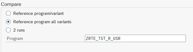
1. Navigate back to the ZRTE_START transaction and choose "Compare runs".
2. Select the comparison mode: "Reference program all variants". This tells RTE to check all established reference points for the specified program.
3. In the "Program" input field, enter the name of your test program ZRTE_TST_R_USR.
4. Execute the comparison (by pressing F8 or clicking the Execute icon).

RTE will now diligently re-execute your program three times, once for each reference variant (ALL, DS, DDIC). It will then compare the data captured during these new executions against the data stored in the corresponding reference runs created moments ago. Logically, since we haven't altered the program's code, the results should perfectly match the references.

Decoding the Comparison Results Grid:

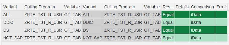
The outcome of the comparison is presented in an ALV grid.

Let's break down the columns and their significance:

• Identifying the Comparison Pair:
  • Left Side (Reference Run Information - light grey background): These columns identify the baseline element of the comparison.
    • Variant : Shows the variant name associated with the reference run.
    • Calling Program : Confirms the program name from the reference run.
    • Variable : Displays the logical name (the IV_VAR_NAME you used in ZCL_RTE=>EXPORT_DATA) of the specific data variable being compared from the reference run.
  • Right Side (New Run Information - darker grey background): These columns identify the run that was just executed for comparison.
    • Variant, Calling Program, Variable : Show the corresponding details for the newly generated run.
    • Observation: In standard "Reference program..." modes, these values should mirror the left side. A discrepancy here (e.g., a variable appearing on the left but not the right) immediately signals that the set of exported variables has changed between the reference capture and the current execution.
• Analysing the Outcome:
  • Result : This column provides the high-level verdict of the comparison for this specific variable pair and comparison type. Possible statuses include:
    • Equal (Highlighted Green): Success! The comparison determined that the data (or structure, depending on the comparison type) is identical between the reference and the new run.
    • Not equal (Highlighted Yellow): A difference was detected. The data or structure does not match. Further investigation is needed.
    • Missing (Highlighted Orange): Indicates that the variable was found and exported in one of the runs (the reference) but was not exported in the other (the new run), or vice-versa. This often points to changes in the program logic controlling the EXPORT_DATA call.
    • Error (Highlighted Red): Signals that the comparison itself could not be successfully performed for technical reasons. The Error column will provide more details.
  • Details : This column becomes active when using the iData comparison type. If iData comparison was performed and the Result is "Not equal", a magnifying glass icon will appear here. Clicking this icon allows you to drill down and see the exact data differences (explored further in section 5.4). For other comparison types or when the result is "Equal", this column is blank and inactive.
  • Comparison : Specifies which type of comparison this particular row in the grid represents. RTE can perform several types of checks configured in the advanced options:
    • RAW data : This is the most basic and fastest comparison. RTE compares serialized values that were saved for the variables. It's a yes/no check – either the values are identical (Equal) or they are not (Not equal). It cannot show what changed, only that a change occurred. Useful for quick checks on large datasets where performance is key.
    • Description : This comparison focuses solely on the structure of the exported variable, not the data values themselves. It checks if elements like field names, data types, field lengths, or the order of fields within an internal table have changed between the reference and the new run. An Equal result means the structure is unchanged; Not equal means the structure has been altered.
    • iData : This is the most powerful and informative comparison type. RTE deserializes the saved raw data back into structured information (like internal tables) for both runs. It then performs a detailed, field-by-field and row-by-row comparison, capable of identifying specific value changes, added rows, or deleted rows. While significantly more resource-intensive and slower than RAW or Description, it's essential for understanding the nature of data differences and enables the drill-down via the Details column.

      Note: iData comparisons do NOT preserve the original order of records. Both tables are sorted before comparison to make it easier to identify differences, such as added or removed records in subsequent runs.

  • Error : If the Result column shows "Error", this column will contain a textual explanation of the problem encountered during the comparison attempt. Common examples include issues with data deserialization or, frequently with iData, an inability to compare due to incompatible data structures between the two runs.

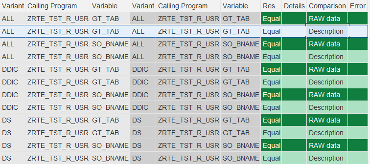
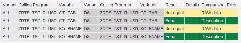
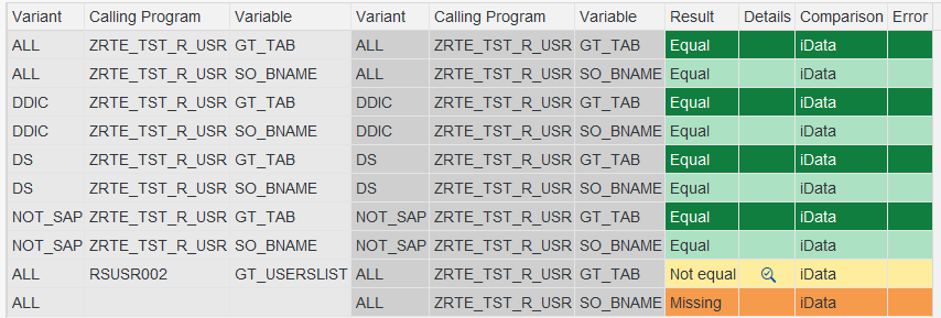
In our initial baseline check we should observe satisfying green "Equal" statuses across the board for both GT_TAB and SO_BNAME for all three variants (ALL, DS, DDIC).

Performance notice. During RTE runs, the variables selected for testing are serialized and stored in the database. During comparisons, this data is retrieved and analyzed. For large datasets, database read/write operations can significantly impact performance. The comparison process may also be memory-intensive, as RTE needs to hold the "before" and "after" states, along with the computed differences — in total, this can require up to three times the size of the original variable state in memory.

Simulating a Code Change

To see how RTE flags discrepancies, let's simulate a simple code change. Imagine we go back into the ZRTE_TST_R_USR program and comment out the specific line responsible for exporting the selection criteria: ZCL_RTE=>EXPORT_DATA( iv_var_name = 'SO_BNAME' i_data = so_bname[] ).. After saving and activating this change, we re-run the "Reference program all variants" comparison.

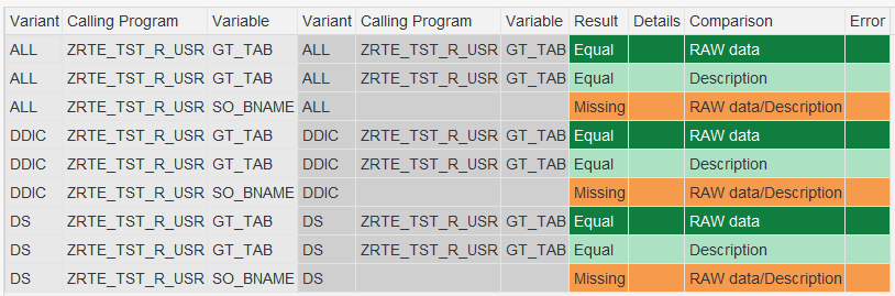
The results grid now tells a different story. For the variable SO_BNAME, the Result column will now display the orange "Missing" status. Furthermore, the right-hand side columns (Variant, Calling Program, Variable) for the SO_BNAME rows will be empty, visually confirming that this variable was present in the reference run (left side) but was not captured in the new execution due to our code change.

5.4 Drilling Down

Let's set up a scenario where we know the data content differs. We'll use the "2 runs" mode to compare the reference run created using the ALL variant against the reference run created using the DS variant. We know these contain different sets of users.

1. Navigate to "Compare runs".
2. Choose the mode: "2 runs".
3. Utilize the search helps provided for the "Run A" and "Run B" fields. For "Run A", locate and select the Run ID corresponding to the reference run of ZRTE_TST_R_USR executed with variant ALL. For "Run B", select the Run ID for the reference run using variant DS.
4. Execute the comparison with default settings.

For the GT_TAB variable, the RAW data comparison will correctly report Result = Not equal, but the Details column will remain inactive, offering no further insight.

Activating and Utilizing the iData Comparison:

To unlock the detailed view, we need to explicitly instruct RTE to perform the iData comparison:

1. On the "Compare runs" selection area, locate and check the "Advanced options" checkbox. This reveals additional control buttons.
2. Click the newly visible "Comparisons" button.
3. A configuration pop-up appears, showing available comparisons. Select "iData", for clarity in this example, you might also unselect "Raw" and "Description". The "iData parameters" button (explained in section 5.5) will also become active if "iData" is selected.
4. Now, re-execute the comparison from the main screen.

The results grid should now reflect that the iData comparison was performed for GT_TAB. The Result will still be "Not equal", but critically, the Details column for that row will now display the magnifying glass icon.

Inspecting the Differences:

This icon is your gateway to understanding the data mismatch. Double-click the magnifying glass icon associated with the GT_TAB comparison row.

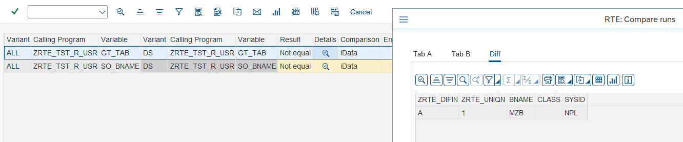
A detailed comparison window pops up, typically featuring three informative tabs:

• Tab A: Displays the complete data content of the GT_TAB variable as captured in the first run you selected (Run A, corresponding to the ALL variant in our case).
• Tab B: Similarly displays the complete data content of GT_TAB as captured in the second run (Run B, corresponding to the DS variant).
• Diff: This is often the most useful tab. It highlights only the discrepancies between Tab A and Tab B. It will clearly mark rows that exist only in Run A, rows that exist only in Run B, or rows with differing field values. In our specific comparison of ALL vs. DS variants, the "Diff" tab should clearly show the user records that are present in the ALL variant's run but were excluded from the DS variant's run.

A Note on Test Data Stability: This example also highlights a crucial aspect of effective regression testing and configuration verification: the stability of your test data environment. If your reference runs capture data that is subject to unrelated changes (like the creation of new users in a development system, or master data changes impacting a configured process), comparisons might frequently show "Not equal" simply because this underlying master data has drifted since the reference run was created. This isn't necessarily a failure of your program code or configuration. Therefore, when designing your test variants and creating reference runs, strive to use selection criteria or data snapshots that are stable or where changes are well understood, allowing you to more clearly isolate differences caused by actual code modifications or intended configuration outcomes.

When results are "Not equal," it's important to analyze whether this is due to an intended code change, a bug, an expected outcome from a configuration change, or an external data factor.

5.5 Handling Differences and Leveraging Data Mapping

Let's walk through how RTE assists in verifying code changes or the impact of configuration adjustments, including situations where the structure of the data itself is modified, necessitating RTE's data mapping capabilities.

Scenario 1: Verifying a Targeted Functional Change

• The Requirement: A new business rule dictates that for the specific administrative user SAP*, the 'CLASS' field in our report's output (GT_TAB) should always display the literal value 'SAP*', overriding whatever value might be stored in the USR02 table. This change should only affect the SAP* user.
• Preparation: To make testing this specific requirement easier, let's first create another variant for our test program. Name it NOT_SAP and configure its selection criteria to include all users except SAP*. Once created, execute the program with this NOT_SAP variant and save it as a reference run. This gives us a baseline that explicitly excludes the user affected by our planned change.
• Implementing the Code Change: Modify the source code of ZRTE_TST_R_USR to implement the hardcoding logic for SAP* 's CLASS field (by uncommenting the code block between tags <2> and </2> in the provided sample program).
• Performing the Regression Test: Go to "Compare runs". Select the "Reference program all variants" mode for ZRTE_TST_R_USR.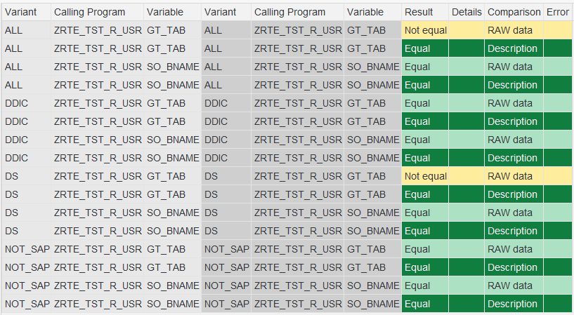
• Analysing the Expected Result: The comparison grid should now clearly demonstrate the impact of our change:
  • For variants ALL and DS (which both include SAP*), the Result for the GT_TAB variable should be "Not equal".
  • Crucially, for variants DDIC and our newly added NOT_SAP (neither of which includes SAP*), the Result for GT_TAB should remain "Equal".
  • This outcome precisely validates our requirement: the change correctly affected only the intended user, and the program's behavior for other user sets remained unchanged, confirming successful regression testing for this modification.

Scenario 2: Dealing with Structural Changes

• The Requirement: A more significant change is requested: we need to add a new column, displaying the user type (USTYP field from USR02), to our main output table GT_TAB.
• Implementing the Code Change: Adjust the program logic to include this new field within the structure and data retrieval for GT_TAB (e.g., by uncommenting the code between tags <3> and </3> and commenting out the original SELECT statement between tags <4> and </4> in the sample program).
• Performing the Test: Use the "Reference program all variants" mode with the iData comparison enabled (see Section 5.4 on how to select iData in "Comparisons" under "Advanced options").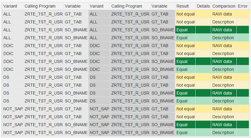 If only RAW Data or Description comparisons are active, you would see the change. However, enabling iData without mapping for a structural change will lead to an error.
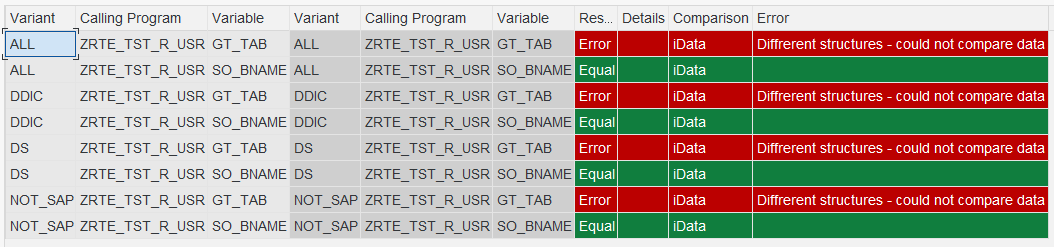
• Observing the Initial Result: This time, the comparison grid presents a different challenge. For the GT_TAB variable, across all variants, you will encounter Result = Error. The corresponding Error column message will read "Different structures - could not compare data". This happens because the fundamental structure of GT_TAB in the reference runs (without USTYP) is inherently incompatible with the structure of GT_TAB in the newly executed runs (which now includes USTYP). RTE's iData comparison, by default, cannot compare tables with different field layouts.

iData Parameters and Mapping

This is where RTE's mapping features become indispensable. They allow you to define rules that tell RTE how to reconcile structural differences before performing the data comparison. The "iData parameters" button becomes available under the "Advanced options" section when iData comparison is active. Clicking this button is your entry point into the mapping configuration.

• Upon clicking "iData parameters", RTE needs to understand the current structure of the variables being exported by the modified program. To achieve this, it automatically re-executes the program for the relevant variants (those selected in 'Reference program/variant' or 'Reference program all variants' modes). This allows it to fetch the latest structural definitions. Be aware that this re-execution step might introduce a noticeable delay before the "iData parameters" window actually appears, especially if the program or variants process large amounts of data. Patience is required here.
• Understanding the "iData parameters" Screen: This screen lists the variable pairs that RTE intends to compare using iData.
  • Include Column: A simple checkbox. Unchecking this will completely exclude the corresponding variable pair (e.g., "SO_BNAME" if we're not interested in it) from the subsequent iData comparison.
  • Prog/Variable A : Identifies the program and variable name originating from the reference run side (Run A).
  • Transform. A : An icon button. Clicking this opens the detailed transformation/mapping editor for the variable(s) from side A.
  • Prog/Variable B : Identifies the program and variable name originating from the newly executed run side (Run B).
  • Transform. B : An icon button, opening the transformation/mapping editor for the variable(s) from side B.
  Grouping: Note that if a specific variable (like GT_TAB) has the exact same structure across multiple reference variants being compared in "Reference program all variants" mode, it will be listed only once on this screen, simplifying the mapping process. (See section 5.5.1 for detailed explanation).

Applying Mapping

Our immediate goal is to compare the data of the original columns, effectively telling RTE to ignore the newly added USTYP column for the purpose of this comparison. This allows us to verify if the data within the pre-existing fields was unintentionally altered by our structural change.

1. On the "iData parameters" screen, locate the row representing the ZRTE_TST_R_USR GT_TAB comparison.
2. Since the structural change (the added USTYP column) occurred in the new execution (Side B), we need to modify its transformation rules. Click the mapping icon button located in the Transform. B column for the GT_TAB row.
3. This action opens the detailed "Transformation" pop-up window for the GT_TAB variable from the new run.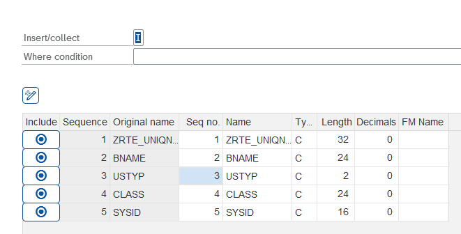
4. Transformation Options: This pop-up is the heart of data mapping in RTE. Let's examine its components thoroughly:
   • Insert/Collect Switch: Allows you to choose the processing logic. Insert (default) treats each row individually. Collect applies ABAP's COLLECT statement logic, which aggregates rows based on non-numeric key fields – useful for specific aggregation scenarios before comparison.
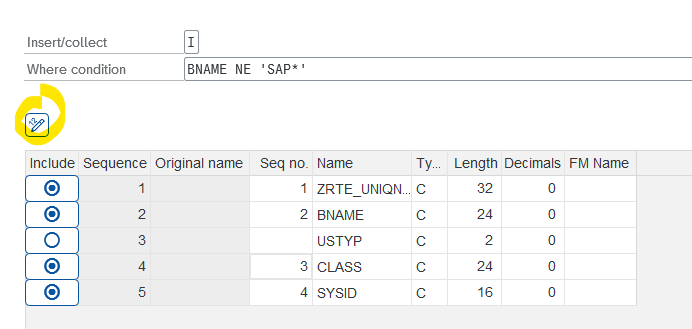
   • WHERE condition Field: A powerful filtering mechanism. Here, you can enter conditions using standard ABAP WHERE clause syntax (but without typing the WHERE keyword itself). For example, BNAME NE 'SAP*' or STATUS EQ 'A' AND VALUE GT 100. RTE performs a syntax check on the condition entered.
   • The Field Mapping Grid: This grid lists all fields present in the variable's current structure (in this case, GT_TAB from the new run, including USTYP). Each row allows detailed control:
     • Include Checkbox: The primary control for including or excluding a specific field from the comparison. If unchecked, the field is completely ignored.
     • Sequence / Original name Columns: These are display-only, showing the field's original position and technical name in the source structure for reference.
     • Seq no. Column: Editable. This numeric field dictates the column order in the final, mapped structure that will be used for the comparison. You can change these numbers to reorder columns.
     • Name Column: Editable. Defines the field name in the mapped structure. This allows you to rename fields if necessary for the comparison (e.g., if comparing MATNR from one table to MATERIAL in another).
     • Type, Length, Decimals Columns: Editable. These allow you to change the data type ('C', 'N', 'P', 'D', 'T', 'STRING', etc.) and corresponding size attributes of a field specifically for the comparison. This is crucial when comparing fields that store similar data but have slightly different technical definitions. Adhere to standard ABAP type definitions. The search help (F4) on the Type field provides guidance on valid types and whether Length/Decimals are applicable. RTE validates these settings and will report errors if inconsistent (e.g., trying to specify a length for a STRING type: For Type g LENGTH must be equal 0, and DECIMALS must be equal 0).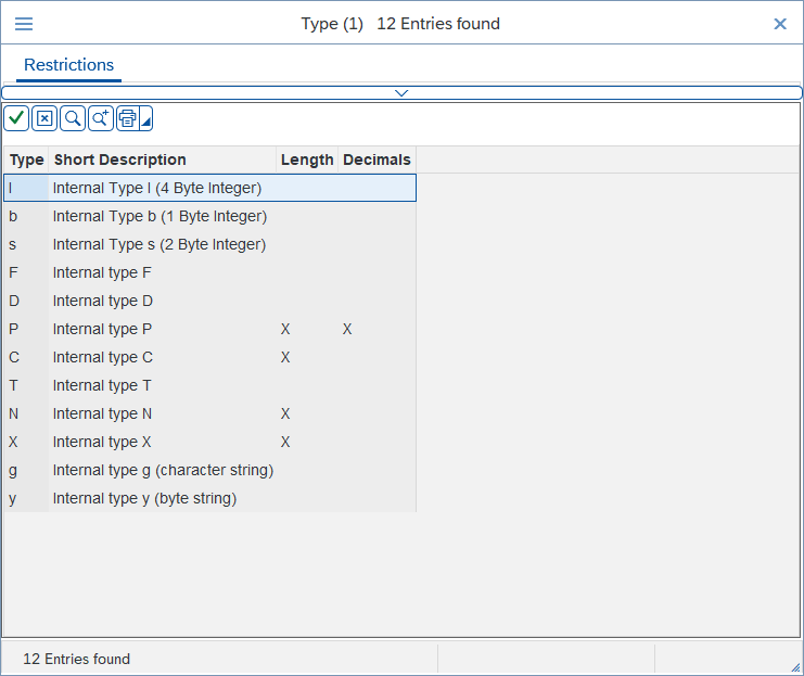
     • FM Name Column: Editable. For advanced scenarios, you can specify the name of a standard SAP conversion exit function module (e.g., CONVERSION_EXIT_ALPHA_INPUT) to transform field values before comparison.
   • Renumerate Button (Pencil Icon): A utility button. After including/excluding fields, clicking this button automatically re-calculates and assigns sequential numbers to the Seq no. column for all included fields, ensuring a clean sequence.
   • OK (Checkmark) / Cancel (X) Buttons: Located at the bottom (OK) or top (Cancel). Use OK to save the mapping changes you've made within this transformation pop-up. Use Cancel to discard them (you will be asked to confirm "Exit without saving?").
5. Applying the Mapping: In our scenario, scroll through the field grid within the "Transformation" pop-up for Transform. B until you find the row representing the newly added field, USTYP . Uncheck the Include checkbox for this specific row.
6. Optionally, click the Renumerate button (pencil icon) to update the Seq no. column for the remaining included fields.
7. Click the OK (Checkmark) button to confirm and close the "Transformation" pop-up, saving the rule to exclude USTYP from side B.
8. You are now back on the main "iData parameters" screen. Click its OK (Checkmark) button to apply all defined parameter settings.
9. Finally, re-execute the comparison from the main "Compare runs" screen.

Interpreting the Result: The comparison for GT_TAB should now proceed without the "Different structures" error. We successfully used mapping to isolate and ignore the structural change, allowing us to focus the comparison on the stability of the original data fields.

Scenario 3: Filtering

Let's revisit Scenario 1 (hardcoding SAP* class) where variants ALL and DS showed Result = Not equal. While this correctly identified the change, perhaps our test goal is to confirm that apart from the intentional change to SAP*, no other users were affected. We can achieve this using mapping filters.

1. Go back to the "Compare runs" screen, ensure "Reference program all variants" and iData comparison are selected.
2. Click on "iData parameters".
3. Locate the row for ZRTE_TST_R_USR GT_TAB. We need to apply a filter to both sides of the comparison to exclude the SAP* user record before the data is compared.
4. Click the Transform. A icon button for GT_TAB. In the "Transformation" pop-up, find the Where condition input field and type the condition: BNAME NE 'SAP*'. Click OK.
5. Click the Transform. B icon button for GT_TAB. In its "Transformation" pop-up, enter the exact same Where condition : BNAME NE 'SAP*'. Click OK.
6. As an optional step, if we are completely uninterested in the SO_BNAME variable for this specific test run, we can uncheck the main Include checkbox for the ZRTE_TST_R_USR SO_BNAME row on the "iData parameters" screen itself. This will skip its comparison entirely.
7. Click OK on the "iData parameters" screen to apply these rules.
8. Re-execute the comparison.

Analysing the Refined Result: Now, when you examine the results grid, the Result for GT_TAB should show "Equal" even for the ALL and DS variants. Why? Because the mapping rules we defined instructed RTE to filter out the SAP* user row from both the reference data and the new run data before performing the comparison. This demonstrates how mapping can be used to focus the comparison and ignore known or intentional differences, allowing you to verify the stability of the remaining data set.

5.5.1 Multiple Variable Entries

As you continue to develop your program and update your reference runs, you might encounter situations where the "iData parameters" screen lists the same logical variable (GT_TAB) multiple times. This occurs when the underlying data structure of that variable has changed over time, and different reference runs (perhaps for different variants, or older vs. newer references for the same variant) capture these different structural versions.

Let's illustrate with an example:

1. Initial State: Suppose you have existing reference runs for several variants (ALL, DS) of ZRTE_TST_R_USR, where GT_TAB has an old structure (without the USTYP field).
2. Structural Code Change: You modify ZRTE_TST_R_USR to add the USTYP field to GT_TAB.
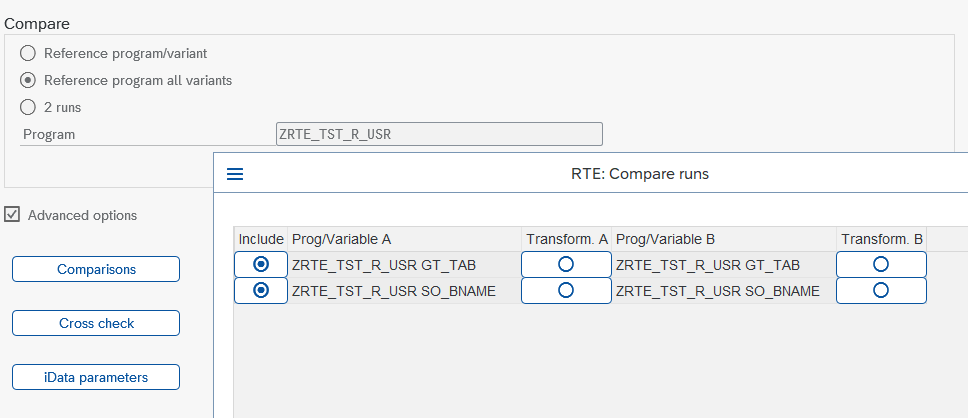
3. Create a New Reference Run: Now, you create a new reference run specifically for the ALL variant. This new reference run for ALL will capture GT_TAB with its new structure (including USTYP). However, the reference run for the DS variant (if not updated) might still be based on the old structure of GT_TAB.
4. Observation in "iData parameters": If you now go to "Compare runs", select "Reference program all variants" (which would include both ALL and DS), and then click the "iData parameters" button, you should see something like :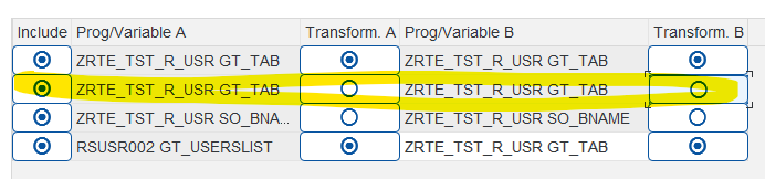

Notice that GT_TAB (from ZRTE_TST_R_USR) appears on multiple lines on both the "Prog/Variable A" (reference) side and the "Prog/Variable B" (current run) side.

Explanation of Multiple Entries:

RTE lists a variable in a new row on the "iData parameters" screen if its underlying data structure is different from other instances of that same logical variable being considered in the current comparison batch.

• Line 1 (representing variant DS): Shows ZRTE_TST_R_USR GT_TAB (from the old reference run of DS, with the old structure) being prepared for comparison against ZRTE_TST_R_USR GT_TAB (from the current execution of the program for DS, which has the new structure). This line would likely require mapping in Transform. A or Transform. B to reconcile the structural differences.
• Line 2 (representing variant ALL): Shows ZRTE_TST_R_USR GT_TAB (from the new reference run of ALL, which has the new structure) being prepared for comparison against ZRTE_TST_R_USR GT_TAB (from the current execution for ALL, also with the new structure).
  • In this specific case (Line 2), because the structure of the reference run (A) now matches the structure of the current run (B), no specific field mapping might be required for this particular pair. The structures are already aligned.

5.6 Cross-Check

One of RTE's most advanced capabilities is the "Cross-Check" feature. This allows you to validate your custom program's output not just against its own previous versions, but against the output of an entirely different program, typically a trusted SAP standard report or a well-established custom tool that performs a similar function. This is invaluable for ensuring your custom development aligns with standard SAP logic or established business processes.

Setting up a Cross-Check:

1. Instrument the Trusted Program: First, you need to ensure the program you want to compare against (the 'reference' program, standard report RSUSR002) also exports the relevant data via RTE. This requires adding a ZCL_RTE=>EXPORT_DATA call at an appropriate point, potentially using SAP's Enhancement Framework if modifying standard code.
   • Example: As shown in the code below, you might create an enhancement implementation at the end of function module SUSR_USERS_LIST_ALV (used by RSUSR002) to export its final user list:

     ENHANCEMENT 1 Z_RTE_EXPORT. "active version
       ZCL_RTE=>EXPORT_DATA( iv_var_name = 'GT_USERSLIST' i_data = gt_userslist ).
     ENDENHANCEMENT.

2. Configure the Cross-Check:
   • Navigate to the "Compare runs" screen. Check the "Advanced options" checkbox.
   • Click the "Cross check" button.
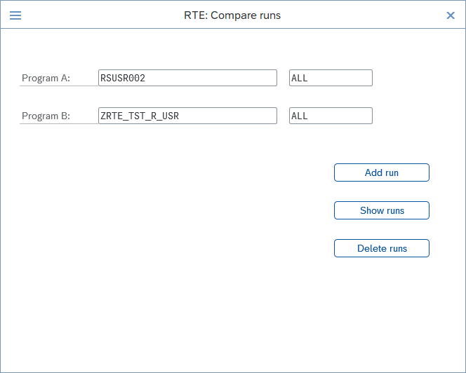
   • A configuration pop-up appears specifically for defining cross-program comparisons.
   • In the Program A row, enter the name and variant of the program you want to use as the reference point (Program: RSUSR002, Variant: ALL).
   • In the Program B row, enter the name and variant of your program under test (Program: ZRTE_TST_R_USR, Variant: ALL). This often defaults based on what you entered on the main comparison screen.
   • Click the "Add run" button. This schedules this specific cross-program comparison pair to be executed. You can add multiple pairs if needed.
   • The "Show runs" button lets you review the list of scheduled cross-checks. The "Delete runs" button clears the entire list if you need to start over.
   • Close the "Cross check" window using the standard close icon (X).

Mapping: The Essential Ingredient for Cross-Checks

Meaningful comparison between two different programs almost always requires data mapping, as it's highly unlikely that the exported variable names, field names, data types, and field order will coincidentally match perfectly.

1. After configuring the cross-check and closing its window, click the "iData parameters" button (ensure iData comparison is selected in "Comparisons").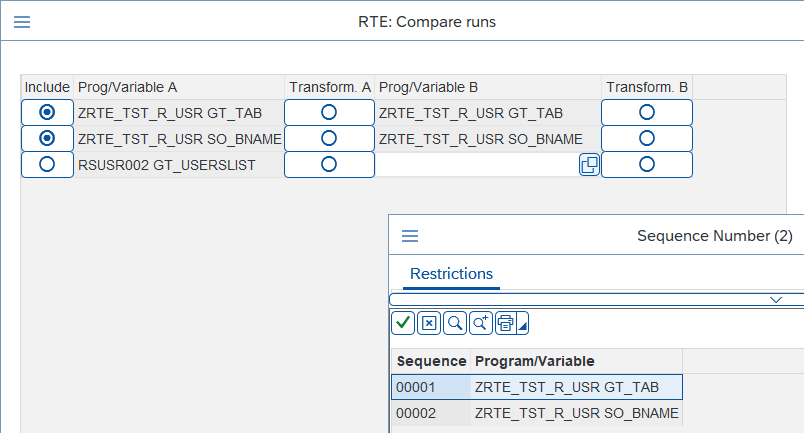
   • The "iData parameters" screen will now list the cross-check pair you scheduled. You'll see the variable exported from Program A (RSUSR002 GT_USERSLIST).
   • However, the Prog/Variable B column for this row will likely be empty initially. RTE cannot automatically guess which variable from Program B should be compared to the variable from Program A. Click the search help icon located within the empty Prog/Variable B field.
   • RTE will present a list of variables exported by Program B (ZRTE_TST_R_USR in our case, showing GT_TAB and SO_BNAME). Select the variable that logically corresponds to the data from Program A (select GT_TAB).
2. Define Transformations: Now you must define mapping rules using the Transform. A and Transform. B buttons to reconcile the differences between RSUSR002 GT_USERSLIST and ZRTE_TST_R_USR GT_TAB.
   • Analyze and Map Transform. A (RSUSR002 GT_USERSLIST): Open its transformation window. Identify the key fields that have equivalents in GT_TAB (BNAME, USTYP, CLASS). Exclude all other fields from GT_USERSLIST that are not relevant for this comparison by unchecking their Include boxes. Use the renumber button to finalize the sequence for side A.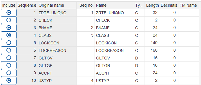
   • Analyze and Map Transform. B (ZRTE_TST_R_USR GT_TAB): Open its transformation window.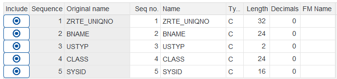
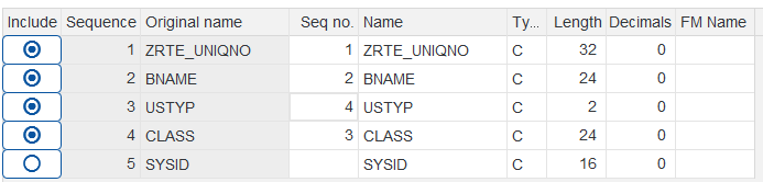
     • Field Matching: Ensure only the fields corresponding to those kept in Transform A are included. Exclude any extra fields unique to GT_TAB (like SYSID).
     • Order Alignment: Adjust the Seq no. values in Transform B so that the order of included fields exactly matches the sequence defined in Transform A (e.g., if A is BNAME, USTYP, CLASS, then B must also be BNAME, USTYP, CLASS in that order). Alternatively, you could adjust A to match B's original order – the key is that the final mapped order is identical on both sides.
     • Type and Length Harmonization: Carefully check the Type, Length, and Decimals of the corresponding fields between A and B. If they differ (e.g., USTYP is C(2) in one and C(4) in the other), you must adjust one side in the mapping to match the other.
       Critical Best Practice: To avoid potential data loss during comparison due to truncation, always modify the field with the shorter length to match the longer length. In the C(2) vs. C(4) example, you should change the C(2) field's mapping definition to C(4), rather than shortening the C(4) field to C(2).
     
3. Once both transformations are defined, click OK on the transformation windows and the main "iData parameters" window.
4. Execute the comparison.

• Interpreting Results: Examine the Result column for the cross-check row. If functional differences exist between the two programs (like our intentional hardcoding of SAP* 's class in ZRTE_TST_R_USR, which differs from RSUSR002 's standard output), you will see "Not equal". Use the Details magnifying glass and the "Diff" tab to pinpoint these functional or configuration-driven discrepancies.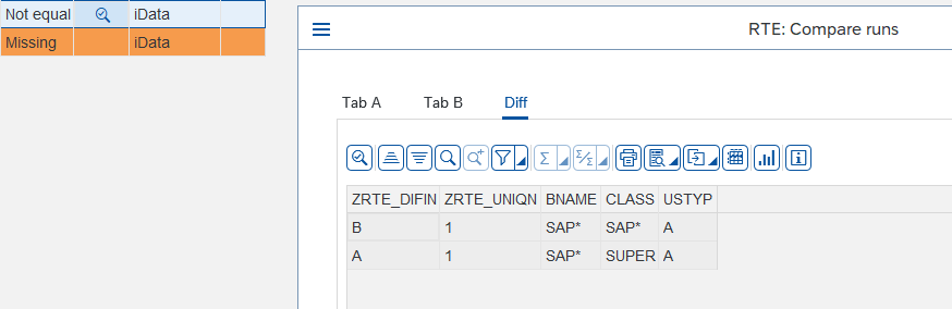
• Refining Comparison: If certain differences are known and accepted (e.g., results of an configuration change expected to differ from the baseline program), you can further refine the comparison by adding appropriate WHERE conditions to both Transform A and Transform B mappings (e.g., adding BNAME NE 'SAP*' to both sides to exclude that specific user from the comparison if it's not relevant to the current check). Remember to save your refined setup as a selection screen variant if you intend to reuse it (see Chapter 5.8 for details).

5.7 Approving New Reference Runs

Development and configuration changes are iterative. After implementing changes (code or configuration), performing comparisons, meticulously analyzing differences using mapping, and ultimately confirming that the program's current behavior is indeed the new correct baseline, your original reference runs might become obsolete. The mappings required to compare against them might become complex and counter-productive for future tests.

RTE provides a streamlined way to update your baseline. Instead of manually re-creating reference runs one by one using the "Run program" transaction, you can approve the runs that were just generated during the comparison process itself, promoting them to become the new official reference runs.

1. Verification is Key: Before proceeding, be absolutely certain that the results shown in your current comparison grid accurately represent the desired, correct state of the program following your latest changes.
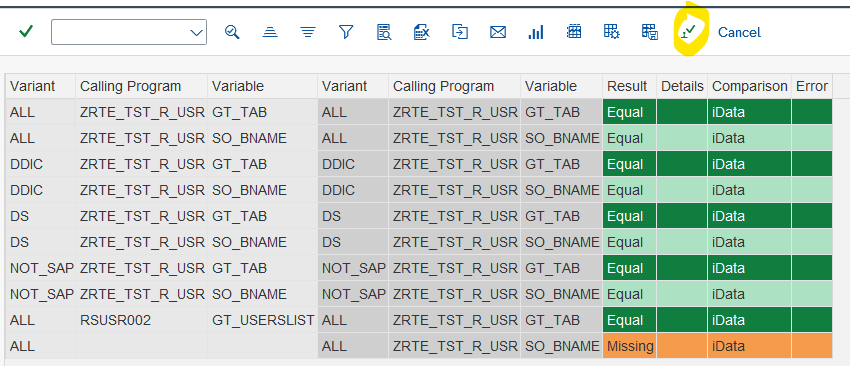
2. Initiate Approval: In the ALV toolbar displaying the comparison results, locate and click the "Approve" button (depicted with a checkmark).
3. Final Confirmation: RTE understands the significance of this action and will present a confirmation pop-up dialog box. It explicitly warns you that clicking "Yes" will designate the runs just executed during the comparison as the new reference runs and, crucially, that this action cannot be undone.
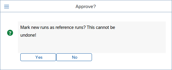
4. Commitment: Only if you are completely confident that the current state is the correct new baseline should you click "Yes".

Consequences of Approval: When you approve, RTE updates its internal records. For each program/variant combination included in the comparison, the run generated during that comparison execution replaces the previous run that was marked as the reference.

Strong Recommendation: Making approval a regular part of your workflow after verifying code or configuration changes is highly recommended, especially following any modifications that alter the structure (fields, types, order) of variables exported via EXPORT_DATA, or after confirming a configuration change has the desired, stable outcome. Approving the new state as the reference significantly simplifies subsequent regression tests or verifications. Future comparisons against this updated reference will start from a structurally identical baseline, reducing or entirely eliminating the need for potentially complex data mappings that were required to bridge the gap with the older, now-obsolete reference run. This keeps your testing process efficient and focused on detecting new, unintended changes.

5.8 Preserving Your Mapping

Configuring intricate mapping rules, especially for complex structural changes or cross-program comparisons, can involve considerable effort. Repeating this setup for subsequent test cycles would be inefficient. RTE provides a standard way to save your entire comparison configuration, including all mapping details, for future use:

• Save Selection Screen Variant: After you have defined your comparison mode, selected programs/runs, and configured all necessary "Advanced options" (including enabling iData, setting up "Comparisons", defining "Cross checks", and meticulously crafting transformations within "iData parameters"), use the standard SAP functionality to save these settings as a selection screen variant for the "Compare runs" screen by clicking the standard Save Variant icon on the toolbar.
• What's Included: Saving a selection screen variant captures the entire state of the "Compare runs" input screen at that moment. This includes:
  • The selected comparison mode (Reference program/variant, All variants, 2 runs).
  • The specified Program names and/or Run IDs.
  • The state of the "Advanced options" checkbox.
  • The selections made within the "Comparisons" pop-up (e.g., which comparison types like iData are active).
  • All defined "Cross check" pairs.
  • The complete "iData parameters" configuration, encompassing which variables are included and, most importantly, all the detailed transformation rules (field inclusions, exclusions, renaming, reordering, type changes, WHERE conditions, conversion exits) defined within Transform. A and Transform. B.
• Reusing Saved Configurations: To reuse a previously saved configuration, simply load the corresponding selection screen variant when you enter the "Compare runs" screen using Get Variant icon. This will instantly restore all your selections and complex mapping settings, saving significant time and effort.
• Important: The saved iData parameters and cross-check definitions within a selection screen variant are intrinsically linked to the specific Program(s) and Variables involved in the comparison when the variant was saved. If you subsequently load a variant but then manually change the primary "Program" name(s) on the selection screen, RTE will automatically clear the restored iData parameters and cross-check definitions associated with the original program(s) from the variant. This is a necessary safety measure, as mappings designed for one program are highly unlikely to be relevant or correct for a completely different program. You would need to redefine the mapping for the new program context.

Chapter 6: Managing Test Runs

Over time, as you conduct numerous tests and verifications, your RTE system will accumulate a history of test runs. The "Manage runs" utility, accessible from the main ZRTE_START transaction, provides a straightforward interface to view the details of these created runs and, importantly, to delete those that are no longer needed, helping to keep your test data repository organized and efficient.

6.1 Selecting Runs

Upon selecting "Manage runs," you are presented with a selection screen that allows you to precisely filter the runs you wish to view or potentially delete.

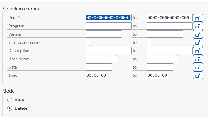
You can specify your search criteria using a combination of the following fields:

• RunID: The unique technical identifier for a run.
• Program: The name of the program for which the runs were executed.
• Variant: The variant used during the run.
• Is reference run?: A checkbox to filter for runs that are (or are not) marked as reference runs.
• Description: The description text provided when the run was created.
• User Name: The SAP user ID of the person who created the run.
• Date: The date on which the run was created.
• Time: The time at which the run was created.

Below the selection criteria, you'll find a "Mode" section with two options:

• View: (Default) Select this mode if you only want to display the details of the runs matching your criteria.
• Delete: Select this mode if your intention is to remove runs from the system.

6.2 Viewing and Deleting Runs

After setting your selection criteria and choosing a mode, executing the screen will display an ALV grid listing all runs that match your input.

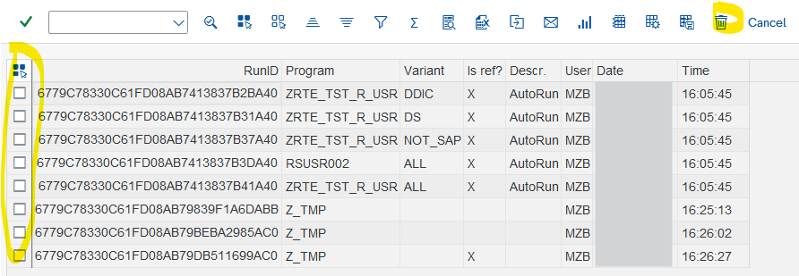
The ALV grid shows the same fields available on the selection screen (RunID, Program, Variant, Is ref?, Description, User, Date, Time), providing a clear overview of each run.

• In View Mode: The ALV simply displays the run information. You can sort, filter the list as needed.
• In Delete Mode:
  • The ALV grid will include selection checkboxes at the beginning of each row.
  • To delete specific runs, check the boxes corresponding to the runs you wish to remove. You can use the standard ALV "Select All" or "Deselect All" buttons for convenience.
  • Once you have selected the runs for deletion, click the trash can icon in the ALV toolbar.
  • RTE will ask for confirmation before permanently deleting the selected runs.

6.3 Recommendations for Managing Runs

Effective management of test runs is important for system performance and clarity.

• In most scenarios, the reference runs are the most valuable ones to keep long-term, as they represent your approved baselines for code or configuration states.
• Periodic Cleanup: It's good practice to periodically review and delete runs that are no longer needed. This typically includes:
  • Old, non-reference runs from previous test cycles.
  • Temporary runs created for ad-hoc investigations.
• Understanding "AutoRun" Descriptions:
  • You might notice runs with "AutoRun" in their Description field. These are runs automatically generated by the "Compare runs" tool when it re-executes programs for comparison (in "Reference program/variant" or "Reference program all variants" modes).
  • An "AutoRun" that is also marked as a reference run (Is ref? = X) indicates that this automatically generated run was subsequently approved by a user via the "Approve" button in the comparison results screen (as detailed in Chapter 5.7).
• Automatic Deletion of Temporary "AutoRuns":
  • By default, the temporary "AutoRun" runs created by the "Compare runs" tool (which are not subsequently approved as reference runs) are automatically deleted when you exit the "Compare runs" screen by using the standard "Back" function that take you back to the main selection screen of "Compare runs" or out of the transaction. This is a cleanup mechanism to prevent an accumulation of temporary comparison data.
  • Important Exception: If you simply close the SAP GUI window of the "Compare runs" results screen without using the standard navigation, these temporary "AutoRuns" will not be automatically deleted.
  • Therefore, to ensure proper cleanup of temporary comparison runs, always use the standard SAP navigation buttons to exit the "Compare runs" functionality.

Regularly using the "Manage runs" tool to clear out obsolete data will help ensure your RTE environment remains lean and focused on the most relevant test information.

Chapter 7: Summary and Cheatsheet

RTE enables a systematic approach to regression testing and configuration verification. Developers or functional consultants instrument code (custom programs or standard SAP programs via enhancements) using ZCL_RTE=>EXPORT_DATA to define test variables. Initial "reference runs" are created via ZRTE_START (transaction "Run program") before code or configuration changes, capturing the baseline state. After modifications or configuration deployment, the "Compare runs" function is used to re-execute the program or compare historical runs, highlighting differences against references. Comparisons include RAW data (fast yes/no check), Description (structure check), and iData (detailed content analysis). For structural changes or cross-program tests, "iData parameters" allow extensive data mapping. If new results are correct and verified, they can be "Approved" as the new reference. "Manage runs" facilitates viewing and deleting old test data. This iterative cycle ensures quality and stability for both development and configuration changes. Key users can also execute comparisons for pre-instrumented programs to validate outcomes.

7.1 RTE Cheatsheet

Here's a quick reference to the most essential RTE elements:

• Key Transaction:
  • ZRTE_START : Central access point (Run program, Compare runs, Manage runs).
• Class ZCL_RTE Methods:
  • EXPORT_DATA( iv_var_name = 'MY_VAR' i_data = lt_data ) : Marks variable for RTE capture.
  • IN_RTE( ) : abap_true if in RTE test; for test-specific logic.
  • COMBINE_DATA( ... ) : Merges data before export (e.g., add context fields).
• "Run Program" Function:
  • Input: Program Name (report, custom or standard), Variant (recommended for repeatability).
  • Mark "Is reference run?" for baselines (unique per program/variant).
  • Disclaimer: RTE doesn't handle program short dumps; ensure program stability.
• "Compare Runs" Function:
  • Modes: Reference program/variant, Reference program all variants, 2 runs.
  • Advanced Options -> Comparisons: RAW data, Description, iData (detailed, enables mapping).
  • Advanced Options -> iData parameters:
    • Include : Toggle variable pair comparison.
    • Transform. A / Transform. B : Opens mapping editor to:
      • Map fields: Include/exclude, reorder, rename, change type/length.
      • Filter rows: Where condition.
      • Aggregate: Insert/Collect.
      • Use FM Name for conversion exits.
  • Advanced Options -> Cross check: Define comparisons between different programs.
  • Approve Button (results ALV): Marks current comparison runs as new references (permanent).
  • Save Comparison Setup: Use "Save Variant" icon on selection screen to save all settings including mappings.
• "Manage Runs" Function:
  • Filter runs by various criteria. Modes: View, Delete.
  • Delete selected runs using trash can icon.
• Critical Reminders & Best Practices:
  • Variants are Key: Ensure consistent test inputs for reliable comparisons.
  • Unique IV_VAR_NAME for Distinct Data: Use unique names for different variables exported in one run. ZRTE_UNIQN handles multiple exports of the same variable.
  • Supported Data Types for Export: Elementary, flat structures, internal tables.
  • Naming IV_VAR_NAME : Follow ABAP variable naming rules (no spaces, limited special chars).
  • Master Data & Test Scenario Stability: Minimize impact by careful variant design.
  • Iterative Approval: Update references after verifying correct changes (code or config).
  • Periodic Cleanup: Use "Manage runs" for old/temporary data.
  • Data Privacy (GDPR): Be mindful if exporting personal data.

Appendix A: Glossary of Terms

• ALV (ABAP List Viewer): Standard SAP framework for displaying lists and tables.
• Cross-Check: An RTE comparison mode where the output of one program is compared against the output of a different program.
• Enhancement Framework: SAP technology allowing modification of standard SAP code using enhancement spots/points. Key for instrumenting standard programs for RTE.
• Export Data (ZCL_RTE=>EXPORT_DATA): The primary RTE method used in ABAP code (standard or custom) to specify which variable's content should be captured by RTE during a run.
• iData Comparison: A detailed comparison type in RTE that deserializes data and performs field-by-field, row-by-row analysis, allowing for difference drill-down and data mapping.
• iData Parameters: A configuration screen in "Compare runs" used with iData comparison to define transformations and mappings for variables.
• Instrumentation: The process of adding ZCL_RTE=>EXPORT_DATA calls (and other optional RTE method calls) to an SAP program (custom or standard) to enable it for testing/verification with RTE.
• IV_VAR_NAME: An input parameter for ZCL_RTE=>EXPORT_DATA that defines the logical name under which a variable's data will be stored and identified within RTE.
• Mapping: The process within RTE (using iData Parameters) of defining rules to reconcile structural or content differences between two data sets before comparison.
• RAW Data Comparison: A fast, yes/no comparison type in RTE that compares the serialized raw data of exported variables.
• Reference Run: A specific execution of a program (usually with a particular variant) captured by RTE that is marked as the "known good" baseline against which future runs are compared.
• Run: A single execution of a program via RTE, during which designated variables are captured and stored.
• RunID: A unique, system-generated technical identifier for each run created by RTE.
• ZRTE_START: The central SAP transaction code for accessing all RTE functionalities.

Appendix B: Common Issues & Troubleshooting

• Program Short Dumps: As stated in section 4.3, RTE does not handle program short dumps. Ensure the program under test is stable. Check transaction ST22 for dump details if a dump occurs.
• EXPORT_DATA Not Capturing Data:
  • Verify the EXPORT_DATA line is actually executed (e.g., using ABAP debugger if necessary).
  • Check if IV_VAR_NAME is unique if multiple distinct variables are exported in the same run.
  • Confirm the data object passed to I_DATA is of a supported type (elementary, flat structure, internal table) and is populated at the point of export.
• "Different structures - could not compare data" in iData Comparison:
  • This is an expected error message if the structure of the exported variable (e.g., fields, field types, field order) has changed between Run A and Run B. This can occur due to code changes or sometimes due to configuration changes that alter output structures.
  • Solution: Use "iData parameters" (Chapter 5.5) to map the fields. You'll need to define transformations for one or both sides (Transform A / Transform B) to:
    • Include/Exclude fields.
    • Rename fields (if logical names differ but content is comparable).
    • Change field types/lengths/decimals for comparison purposes.
    • Reorder fields so that the mapped structures become compatible for comparison.
• Variant Not Found:
  • Double-check the spelling of the variant name.
  • Ensure the variant exists for the specified program in the current SAP system and client. Variants are client-specific.
• Unexpected "Not Equal" Results in Comparison:
  • Always use the iData comparison type and drill down using the magnifying glass icon in the Details column to see the "Diff" tab. This will show exact data differences.
  • Consider the cause:
    • Is it an intended code change? If so, the result might be correct.
    • Is it a bug in the program?
    • Is it an expected outcome from a recent configuration change?
    • Is it due to underlying master data changes in the test system?
• Delay when opening "iData parameters":
  • As noted in section 5.5, RTE will re-execute the program to determine current data structures. This can take time for programs processing large data volumes. Please be patient.